
All you need to know about Linear Regression
Reading outcomes
- Understanding why Linear Regression is a supervised ML algorithm.
- Noting the assumptions made by the algorithm.
- A problem where linear regression might be applicable.
- Deriving the loss function both by intuition and by probabilistic methods.
- Math for fun.
Problem setup, Hypothesis
Linear Regression is one of the supervised learning algorithm that models the relationship between label y and inputs X.
Let’s consider high school math where we had equation of a line like so,
\[\mathbf{y} = \mathbf{mx + b}\]where, y is linear combination of inputs X m is slope and b is the y intercept
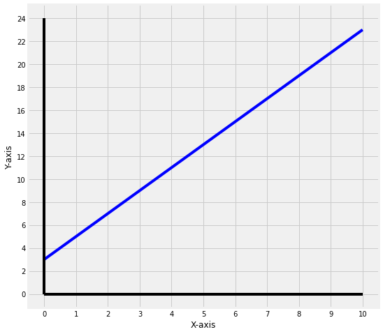
The above figure is a plot of the equation,
\[\mathbf{y} = \mathbf{2x} + \mathbf{3}\]So, we can safely say that, the slope or m is 2 which means for each unit change in x there will be 2 unit changes in y i.e \(\Delta y/\Delta x = 2\). And the y intercept or b = 3, so the line will always pass through \(y = 3\).
We use a similar equation when creating a machine learning linear regression model. Before trying to use a model for a machine learning problem, it is essential to understand the assumptions made by the algorithm about the data.
Assumptions
- Linear Regression assumes that the data points are continuous. If we look at the above above figure, we can see that the values are continuous and not discrete.
- Linear Regression assumes that the labels are a function of the linear combination of the inputs and a normally distributed error term or gaussian noise. (Please ignore the normally distributed error term part if you are a beginner, it is not required to get an intuitive understanding of the workings)
These assumptions are one of the most critical elements in the machine learning task. It actually helps us understand the data well. To put it in other words, before using a machine learning algorithm on a dataset, one must understand the data using some exploratory data analysis (EDA), only when you’re convinced about an algorithm being useful on a particular dataset should you go ahead and use it.
There is a fair argument that we can possibly throw all the algorithms at the data and figure out which one gives a better result. Try saying this in an interview and look where this goes. My personal opinion is to always keep constraints in mind when developing products and writing code and build on from there. In our case, data is the constraint and hence we should check the assumptions made by the algorithm, do our EDA and choose a suitable algorithm.
Example
Let’s use a dataset that obeys the above assumptions.
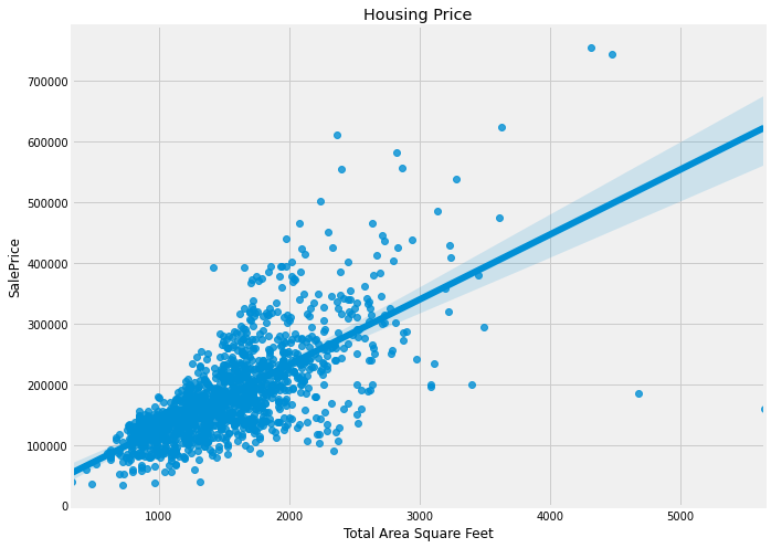
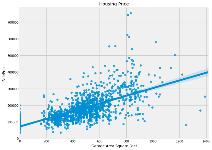
The housing dataset on Kaggle is a good example of when one can use linear regression to predict price of house given a lot of information about the house like total area, whether the house has a garage or not, total rooms, etc
The features like garage area and ground floor area seem to fit our expectation pretty well. The charts were drawn using Seaborn which is an API wrapper over the Matplotlib library.
Now that we have an example in picture let’s move to the loss function and other important mathematical details about Linear Regression.
Loss Function
Now, if we want that given a data point, or given garage area, we should be able to correctly predict the house price.
So, we first need to find out the values of m and b. We can then plug in the values in the equation \(y = m*x + b\) and get out Sale Price i.e. y.
Using Machine Learning, we exactly do this, find/learn the values of m and b.
Going back, let’s say our linear function which maps y to X is f. So we can say that,
\(\mathbf{y} = \mathbf{f(X)}\) .. (remember y = mx + b)
Intuitively, we know that if we want our prediction to be correct,
the original value of y should be as close to value given by f(x) i.e. put mathematically, we can say,
\(\mathbf{y} - \mathbf{f(X)} = \mathbf{0}\) ..(this is the optimal condition, but even if it is close to 0, it’s good)
Now, if we calculate this value for all the examples, we have a sum error i.e. error of summing the y - f(X) for all examples. Can be called sum of errors.
However, y - f(X) can be negative if our prediction is more than original value, it can also be positive if our prediction is less than y, so if we cannot just sum them, we have to take absolute values so that the negative and positive values do not cancel each other out. By calculating a mean of that, we get the mean error.
Mathematically,
\[error = {1\over n} * | \sum y - f(X) |\]where n = total number of points
However, we do a small trick here to penalize the huge errors using squared sum of errors, we can talk about that later in another post. The function changes to,
mean squared error = \({1\over n} * (\sum y - f(X))^2\)
This function is called the loss function and written in more complicated way is written as,
\[MSE = (\frac{1}{n})\sum_{i=1}^{n}(y_{i} - x_{i})^{2}\]Finally, some prefer to take a Root mean squared error rather than the mean squared error. Because why not? If it works for squares, should work for square roots as well, and the value would be smaller too.
\[RMSE = \sqrt{(\frac{1}{n})\sum_{i=1}^{n}(y_{i} - x_{i})^{2}}\]Some more math for fun
Note: Derivation for the above loss function, the probabilistic way.
Let’s say w is the weights or parameters that we want to learn (remember m and b). So, the objective function is given by,
\[\mathbf{w} = \underset {x} {\arg\max} P(y_1,\mathbf{x}_1,...,y_n,\mathbf{x}_n|\mathbf{w})\]What does this mean?
Maximize the probability of y being correct (as correct as possible); given the data points. Or even simply, give me the best prediction of y when values of X are given.
Objective Function: The function that shows our objective of wanting to reduce the error of the RMSE or MSE.
The probabilities are products, we assume independence of probabilities between different features and use the chain rule of probability and finally as usual, we assume the probability distribution is gaussian in nature. Hence, the above equation becomes,
\[\mathbf{w} = \underset {x} {\arg\max} \sum_{i=1}^n \left[\frac{1}{\sqrt{2\pi\sigma^2}} \left(e^{-\frac{(\mathbf{x}_i^\top\mathbf{w}-y_i)^2}{2\sigma^2}}\right)\right]\]Now again, we take the logs, eliminate the constant on the left and take a derivative, and because there is a minus sign, the arg max is converted to arg min, and finally the equation becomes something we have seen before,
\[\mathbf{w} = \underset {x} {\arg\min} \frac{1}{n}\sum_{i=1}^n (\mathbf{x}_i^\top\mathbf{w}-y_i)^2\]Remember the MSE from before, the only change is f(x) now becomes \(X^TW\) which is nothing but again a linear combination of weights and input matrix like we discussed before.
Closed form
Now, only for Linear Regression, there is a closed form formula which can be directly used to calculate the model parameters or coefficients or W.
\[\theta = {(\mathbf{X^TX})^{-1}}\mathbf{X}\mathbf{y}\]Check the code below, that finds parameter \(\theta\). Here, for simplicity, I have used a single dimensional input.
So, even without any learning system, we can find that X and y are related to each other. The value of y is 10 times the value of X i.e. our parameter \(\theta\) is 10.
You can read about the derivation here.
So, we actually do not learn anything, just do the above matrix calculations and we get the coefficients or weight matrix.
Awesome right? Yes, but not always!
Some questions to think about
Q1. If we have the closed form, why bother learning the weights?
If the dimensionality of inputs is huge and we have lot of data points, we might run into computational troubles. We first take a dot product of the inputs X and then calculate the inverse and some other computation. This is quite expensive. So, the closed form might not always be a best idea.
Q2. Can we do anything better to learn the parameters iteratively?
Enter Gradient Descent. We will look into Gradient Descent and how its variants can be used to learn the parameters iteratively in one of the following posts.
Spoiler: What we end up doing is essentially learn the parameters of the model slowly using Gradient Descent rather than using the closed form to calculate them.
Leave a comment