
All you need to know about kNN (k Nearest Neighbors)
What are the learning outcomes after reading the post?
I assume that you have a fair bit of understanding of the Machine Learning world. After the reading this post, you will be able to answer below questions:
- What are the types of problems where kNN algorithm can be used?
- What are the assumptions made by the kNN algorithm?
- What are the hyper-parameters and its significance?
- How the curse of dimensionality curse this algorithm?
In short, one is probably asked these questions in an interview to gauge the understanding if at all the interviewer is interested in the kNN algorithm.
What is the kNN algorithm?
A supervised machine learning algorithm that can be used to solve both classification and regression problems. It uses the neighbourhood to predict where a test point might belong.
kNN as a classification problem
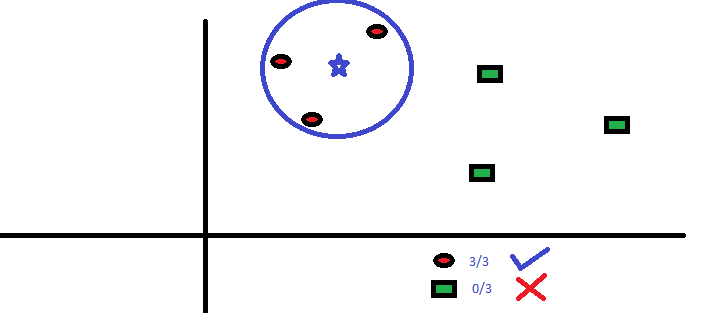
In the image above we can see that the test point, denoted by a star uses the neighbours to classify itself as a red circle and not the green square. Since we are classifying the blue star in one of red circle or green square classes, it is a classification problem.
kNN as a regression problem
Suppose in the above image, the red circles and green squares are replaced with solid black circles and have some real values. Then by averaging the closest values to the new test data point, we can find it’s predicted value. This slight modification makes it a regression problem.
Instance-based or Lazy learner
Most people who have practiced machine learning know that there are 2 major phases amongst others.
- Training phase
- Testing phase
Most of the algorithms learn a representation of the input X -> output Y, i.e. Y = f(X) during the training phase.
The kNN algorithm unlike most other algorithms does not actually learn anything during the training phase. It just memorises the training examples. It is during the testing phase that it evaluates how close are the testing examples to the stored training examples. And hence, the algorithm is called a lazy or instance based learner.
Hyper-parameters
The only hyper-parameter in the algorithm is the value of k i.e. the number of neighbours to evaluate against.
Role of 'k' in Bias and Variance
Low k => High Variance
High k => High Bias
What does this mean?
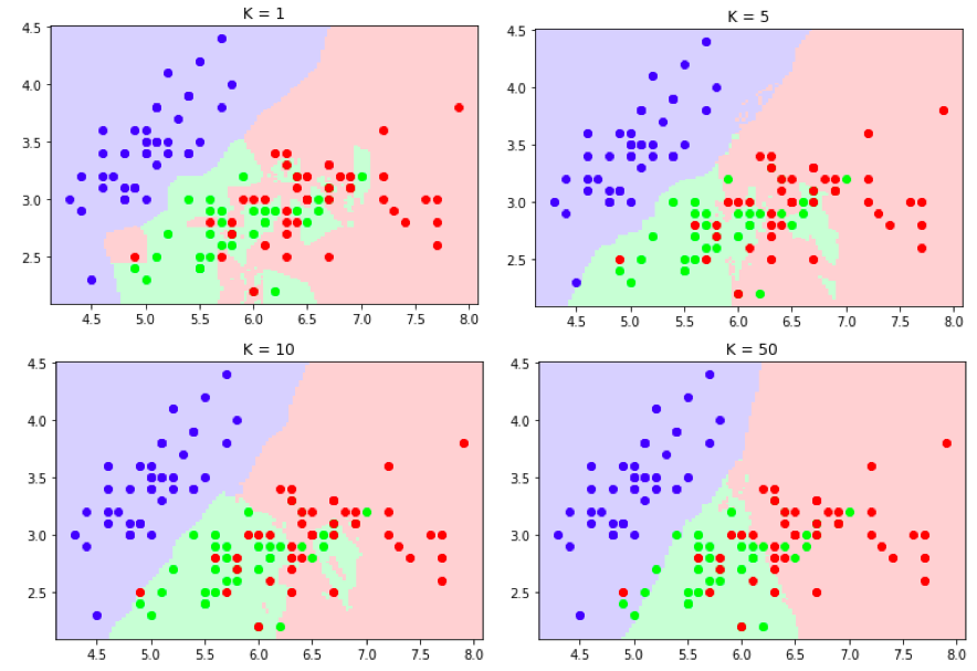
In the above image, when k=1, the decision boundary seems to be very picky i.e. it does not miss even a single point and considers it to be the neighbourhood.
When k=5 and k=10, the red point to the lower left is classified as green and quite a few others are mis-classified as well.
When k=50, the boundaries look real as if there are some clear clusters and the points have though mis-classified seem ok.
Now, what are the mistakes one can do in understanding the decision boundaries?
- In the above example, we saw that the k=50 which was the highest gave us a robust decision boundary. However, one should understand that a high value of
kis not always desirable. A very high value ofkusually means there is high information loss and that a lot of points might be mis-classified. This phenomenon is also called High Bias. - Also, when k=1, we saw the boundaries did not make a lot of sense because each point had been marked equally important which might not be the case. In real life there are issues like mis-labelling, anomalies in data, errors in data collection, etc which might have caused some points to fall in the wrong class. Hence, it is also not advised to use very low
k. This phenomenon is also called High Variance.
Finally, we should ideally experiment with values of k and choose one that has neither high bias or high variance.
Train, Test, Validation set
We saw above that the value of k should neither result in high bias or in high variance. But, how to choose such a value of k?
Suppose that our data set has 100 data points. We break the data set like shown below:
- 70 => train
- 15 => validation
- 15 => test
The train chunk is used for training (in this case, just storing), the valid chunk is used for tuning the hyper-parameters (in this case, k). So, we check for each value of k in a range, how our classification algorithm performs. When we are sure of the best k, we use the model to test our real performance using the unseen test set.
So, why not use only train and test set? Why is validation set required?
When we tune our model based on different values of k, we use the validation set and our results might be biased towards the validation set. In a real life scenario, though the distribution of the train and test set are expected to be similar, the new data might be unseen and the algorithm should be able to make correct classification based on previous data and not just be biased towards previously seen data. Hence, an additional validation set is essential.
Below is an image that will be helpful in understanding what is a correct way to tune the hyper-parameter.
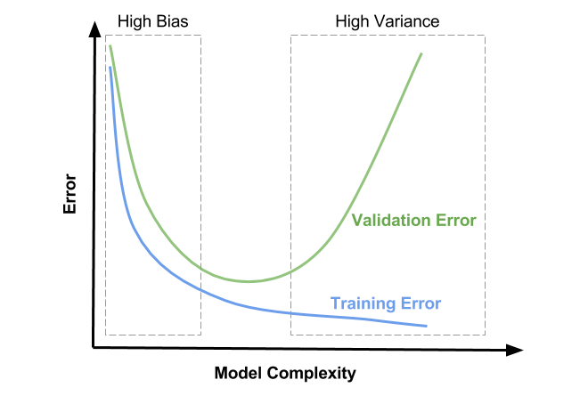
In the image, the value of training and validation error reduce sharply in the beginning, and almost plateau in the range between and High Bias and High Variance boxes and then even though the training error seems to be reducing, the validation error keep increasing. We have be somewhere in between the boxes where the difference in training and validation errors are the minimum.
Role of the Distance metric
The semantic meaning between data points is established by using the distance metric. In simple terms, it is the distance measure which gets to decide (indirectly) which data points are similar and which are not. Now, consider a case where data has N dimensions. One of them is height in meters (0-2 m) and the other is weight in pounds (0-500 lbs). Suppose we choose the Euclidean distance as the metric.
\[d\left(X_{1},X_{2}\right) = \sqrt {\sum _{i=1}^{n} \left( X_{1_i}-X_{2_i}\right)^2 }\]Since the Euclidean computes the squared difference, the larger valued features will be favoured and important information from other features might be lost. The model might learn the wrong function that maps the input to output which in turn might lead to incorrect predictions (accuracy). Hence, choosing a correct distance metric is very important when using the kNN algorithm.
Assumptions the algorithm makes
Probably the most important aspect of choosing an algorithm to fit a problem is knowing what underlying assumptions the algorithm makes about the data set.
The kNN algorithm has one very essential assumption about the data set. It is
Similar inputs have similar labels
What does this mean?
If 2 data points have similar labels, it is inferred that they must have been same. Example: If you want to detect whether a particular picture has a dog or a cat, kNN is a possible candidate to be chosen as a learner. However, if there are quite a few dog breeds in the data set and they have very different characteristics, then kNN might not be the optimal choice.
Why is it so?
The assumption is that 2 dogs have similar features. However, due to the background, body features of the dog, color, etc; the dogs might actually be quite different from each other and hence the kNN algorithm might fail.
So where will it shine?
Consider you have a lot of photos in your gallery which includes your individual pictures and ones along with your friends and family as well. Now, most of your photos will have same characteristics. So, you can train an algorithm to detect if you are present in a particular picture.
What do you mean by features?
Your face has typical features like the shape of your nose, some spots on the skin, thickness of the eye bros, hair style, lips, etc. These are all captured in a picture in pixels. So, if these pixels have similar properties in different photos, the algorithm might be able to learn that they belong to you and hence recognise you when a new picture of you is shown.
Note: The pixels are arranged as one long vector and hence do not actually capture the contextual information like the distance between your eyes OR symmetry of the face, etc. For such advanced cases, a neural network based architecture called the Convolutional Neural Networks (CNNs) are more useful and robust.
The curse of dimensionality
Based on the assumption that, “Similar inputs have similar labels”, we can say one thing, “The algorithm will try to match all the input dimensions to draw inferences”. So, if one has 1000 features or input dimensions, the algorithm will be checking each and every one of them. Below are the problems due to that:
- Some features might be important and still be consider equally important to other important features. Ex: The corners of photos might not be as important as the center but the algorithm might weigh them to be equal
- Based on the above point we can say that, as the number of features OR dimensions increase, the data points will start getting more dissimilar to each other
- As the number of dimensions and number of examples increases, the algorithm will get slower. Add to that the fact that the algorithm will be storing the examples rather than learning a function.
Enhancing kNN
Using a data structure that can store indices such that not all the points have to be compared to find the k closest ones. The data structure is called a kd tree which acts as an index. We
form bins that have similar data points and instead of comparing all the data points, we can compare the test data point with the bin value and determine the closest ones.
Leave a comment